Sabado, Oktubre 11, 2014

First Order Circuits

First order circuits are circuits that contain only one energy storage element (capacitor or inductor), and that can, therefore, be described using only a first order differential equation. The two possible types of first-order circuits are:

RC (resistor and capacitor)

RL (resistor and inductor)

RL and RC circuits is a term we will be using to describe a circuit that has either a) resistors and inductors (RL), or b) resistors and capacitors (RC).

RL Circuits

An RL Circuit has at least one resistor (R) and one inductor (L). These can be arranged in parallel, or in series. Inductors are best solved by considering the current flowing through the inductor. Therefore, we will combine the resistive element and the source into a Norton Source Circuit. The Inductor then, will be the external load to the circuit. We remember the equation for the inductor:

$v(t) = L\frac{di}{dt}$

If we apply KCL on the node that forms the positive terminal of the voltage source, we can solve to get the following differential equation:

$i_{source}(t) = \frac{L}{R_n}\frac{di_{inductor}(t)}{dt} + i_{inductor}(t)$

RC Circuits

An RC circuit is a circuit that has both a resistor (R) and a capacitor (C). Like the RL Circuit, we will combine the resistor and the source on one side of the circuit, and combine them into a thevenin source. Then if we apply KVL around the resulting loop, we get the following equation:

$v_{source} = RC\frac{dv_{capacitor}(t)}{dt} + v_{capacitor}(t)$

First Order Solution

Series RL

The differential equation of the series RL circuit

$L \frac{dI}{dt} + I R = 0$

$\frac{dI}{dt} = - I \frac{R}{L}$

$\frac{1}{I} dI = - \frac{R}{L} dt$

$\int \frac{1}{I} dI = - \frac{R}{L} \int dt$

$ln I = - \frac{R}{L} t + C$

$I = e^(- \frac{R}{L} t + C )$

$I = A e^(- \frac{R}{L} t )$

Series RC

The differential equation of the series RC circuit

$C \frac{dV}{dt} + \frac{V}{R} = 0$

$\frac{dV}{dt} = - V \frac{1}{RC}$

$\frac{1}{V} dV = - \frac{1}{RC} dt$

$\int \frac{1}{V} dV = - \frac{1}{RC} \int dt$

$ln V = - \frac{1}{RC} t + C$

$V = e^(- \frac{1}{RC} t + C )$

$V = A e^(- \frac{1}{RC} t )$

Time Constant

The series RL and RC has a Time Constant

$T = \frac{L}{R}$

$T = \frac{RC}{1}$

In general, from an engineering standpoint, we say that the system is at steady state ( Voltage or Current is almost at Ground Level ) after a time period of five Time Constants.

Overview and Insights

First order circuit is a circuit that only contain one energy storage element, that is a capacitor or an inductor.
There are only two possible first order circuits, the RC (Resistor and Capacitor) & RC (Resistor and Inductor).
The time constant is the same regardless of what the output is defined to be.
When a circuit has a capacitor/inductor, a resistor and a dependent source. We use Thevenin's theorem and its equivalent can be found at the terminals of a capacitor or an inductor.

Maximum Power Transfer Theorem, Capacitors and Inductors

Maximum Power Transfer Theorem

The Maximum Power Transfer Theorem is not so much a means of analysis as it is an aid to system design. Simply stated, the maximum amount of power will be dissipated by a load resistance when that load resistance is equal to the Thevenin/Norton resistance of the network supplying the power. If the load resistance is lower or higher than the Thevenin/Norton resistance of the source network, its dissipated power will be less than maximum.

This is essentially what is aimed for in radio transmitter design , where the antenna or transmission line “impedance” is matched to final power amplifier “impedance” for maximum radio frequency power output. Impedance, the overall opposition to AC and DC current, is very similar to resistance, and must be equal between source and load for the greatest amount of power to be transferred to the load. A load impedance that is too high will result in low power output. A load impedance that is too low will not only result in low power output, but possibly overheating of the amplifier due to the power dissipated in its internal (Thevenin or Norton) impedance.

Taking our Thevenin equivalent example circuit, the Maximum Power Transfer Theorem tells us that the load resistance resulting in greatest power dissipation is equal in value to the Thevenin resistance (in this case, 0.8 Ω):

With this value of load resistance, the dissipated power will be 39.2 watts:

The Maximum Power Transfer Theorem is not: Maximum power transfer does not coincide with maximum efficiency. Application of The Maximum Power Transfer theorem to AC power distribution will not result in maximum or even high efficiency. The goal of high efficiency is more important for AC power distribution, which dictates a relatively low generator impedance compared to load impedance.

Similar to AC power distribution, high fidelity audio amplifiers are designed for a relatively low output impedance and a relatively high speaker load impedance. As a ratio, "output impdance" : "load impedance" is known as damping factor, typically in the range of 100 to 1000. [rar] [dfd]

Maximum power transfer does not coincide with the goal of lowest noise. For example, the low-level radio frequency amplifier between the antenna and a radio receiver is often designed for lowest possible noise. This often requires a mismatch of the amplifier input impedance to the antenna as compared with that dictated by the maximum power transfer theorem.

Capacitors

Just like the Resistor, the Capacitor, sometimes referred to as a Condenser, is a simple passive device that is used to “store electricity”. The capacitor is a component which has the ability or “capacity” to store energy in the form of an electrical charge producing a potential difference (Static Voltage) across its plates, much like a small rechargeable battery.

There are many different kinds of capacitors available from very small capacitor beads used in resonance circuits to large power factor correction capacitors, but they all do the same thing, they store charge.

In its basic form, a Capacitor consists of two or more parallel conductive (metal) plates which are not connected or touching each other, but are electrically separated either by air or by some form of a good insulating material such as waxed paper, mica, ceramic, plastic or some form of a liquid gel as used in electrolytic capacitors. The insulating layer between a capacitors plates is commonly called the Dielectric.

Due to this insulating layer, DC current can not flow through the capacitor as it blocks it allowing instead a voltage to be present across the plates in the form of an electrical charge.

Inductors

An inductor is a passive electronic component that stores energy in the form of a magnetic field. In its simplest form, an inductor consists of a wire loop or coil. The inductance is directly proportional to the number of turns in the coil. Inductance also depends on the radius of the coil and on the type of material around which the coil is wound.

For a given coil radius and number of turns, air cores result in the least inductance. Materials such as wood, glass, and plastic - known as dielectric materials - are essentially the same as air for the purposes of inductor winding. Ferromagnetic substances such as iron, laminated iron, and powdered iron increase the inductance obtainable with a coil having a given number of turns. In some cases, this increase is on the order of thousands of times. The shape of the core is also significant. Toroidal (donut-shaped) cores provide more inductance, for a given core material and number of turns, than solenoidal (rod-shaped) cores.

The standard unit of inductance is the henry, abbreviated H. This is a large unit. More common units are the microhenry, abbreviated µH (1 µH =10^-6H) and the millihenry, abbreviated mH (1 mH =10^-3 H). Occasionally, the nanohenry (nH) is used (1 nH = 10^-9 H).

It is difficult to fabricate inductors onto integratedcircuit (IC) chips. Fortunately, resistors can be substituted for inductors in most microcircuit applications. In some cases, inductance can be simulated by simple electronic circuits using transistors, resistors, and capacitors fabricated onto ICchips.

Inductors are used with capacitors in various wireless communications applications. An inductor connected in series or parallel with a capacitor can provide discrimination against unwanted signals. Large inductors are used in the power supplies of electronic equipment of all types, including computers and their peripherals. In these systems, the inductors help to smooth out the rectified utility AC, providing pure, battery-like DC.

Overview and Insights

The Maximum Power Transfer Theorem states that the maximum amount of power will be dissipated by a load resistance if it is equal to the Thevenin or Norton resistance of the network supplying power.
The Maximum Power Transfer Theorem does not satisfy the goal of maximum efficiency.
The SI unit of capacitance is the farad [F], which is equivalent to the coulomb per volt [C/V].
One farad is generally considered a large capacitance.
The energy stored in a capacitor can be calculated using one of the following equations …
Inductors can be connected together in either a series connection, a parallel connection or combinations of both series and parallel together, to produce more complex networks whose overall inductance is a combination of the individual inductors. However, there are certain rules for connecting inductors in series or parallel and these are based on the fact that no mutual inductance or magnetic coupling exists between the individual inductors.

Thevenin's and Norton's Theorem

Thevenin’s Theorem and Norton’s Theorem

Thevenin's Theorem

Thevenin's Theorem states that it is possible to simplify any linear circuit, no matter how complex, to an equivalent circuit with just a single voltage source and series resistance connected to a load. The qualification of “linear” is identical to that found in the Superposition Theorem, where all the underlying equations must be linear (no exponents or roots). If we're dealing with passive components (such as resistors, and later, inductors and capacitors), this is true. However, there are some components (especially certain gas-discharge and semiconductor components) which are nonlinear: that is, their opposition to current changes with voltage and/or current. As such, we would call circuits containing these types of components, nonlinear circuits.

Thevenin's Theorem is especially useful in analyzing power systems and other circuits where one particular resistor in the circuit (called the “load” resistor) is subject to change, and re-calculation of the circuit is necessary with each trial value of load resistance, to determine voltage across it and current through it. Let's take another look at our example circuit:

Let's suppose that we decide to designate R2 as the “load” resistor in this circuit. We already have four methods of analysis at our disposal (Branch Current, Mesh Current, Millman's Theorem, and Superposition Theorem) to use in determining voltage across R2and current through R2, but each of these methods are time-consuming. Imagine repeating any of these methods over and over again to find what would happen if the load resistance changed (changing load resistance is very common in power systems, as multiple loads get switched on and off as needed. the total resistance of their parallel connections changing depending on how many are connected at a time). This could potentially involve a lot of work!

Thevenin's Theorem makes this easy by temporarily removing the load resistance from the original circuit and reducing what's left to an equivalent circuit composed of a single voltage source and series resistance. The load resistance can then be re-connected to this “Thevenin equivalent circuit” and calculations carried out as if the whole network were nothing but a simple series circuit:

. . . after Thevenin conversion . . .

Norton's Theorem

Norton's Theorem states that it is possible to simplify any linear circuit, no matter how complex, to an equivalent circuit with just a single current source and parallel resistance connected to a load. Just as with Thevenin's Theorem, the qualification of “linear” is identical to that found in the Superposition Theorem: all underlying equations must be linear (no exponents or roots).

Contrasting our original example circuit against the Norton equivalent: it looks something like this:

. . . after Norton conversion . . .

Remember, the arrow notation for a current source points in the direction opposite that of electron flow. Again, apologies for the confusion. For better or for worse, this is standard electronic symbol notation.

Overview and Insights

Thevenin's Theorem is a way to reduce a network to an equivalent circuit composed of a single voltage source, series resistance, and series load.
Steps to follow for Thevenin's Theorem:

(1) Find the Thevenin source voltage by removing the load resistor from the original circuit and calculating voltage across the open connection points where the load resistor used to be.

(2) Find the Thevenin resistance by removing all power sources in the original circuit (voltage sources shorted and current sources open) and calculating total resistance between the open connection points.

(3) Draw the Thevenin equivalent circuit, with the Thevenin voltage source in series with the Thevenin resistance. The load resistor re-attaches between the two open points of the equivalent circuit.

(4) Analyze voltage and current for the load resistor following the rules for series circuits.

Norton's Theorem is a way to reduce a network to an equivalent circuit composed of a single current source, parallel resistance, and parallel load.
Steps to follow for Norton's Theorem:

(1) Find the Norton source current by removing the load resistor from the original circuit and calculating current through a short (wire) jumping across the open connection points where the load resistor used to be.

(2) Find the Norton resistance by removing all power sources in the original circuit (voltage sources shorted and current sources open) and calculating total resistance between the open connection points.

(3) Draw the Norton equivalent circuit, with the Norton current source in parallel with the Norton resistance. The load resistor re-attaches between the two open points of the equivalent circuit.

(4) Analyze voltage and current for the load resistor following the rules for parallel circuits.

Lunes, Agosto 25, 2014

Superposition Theorem

Superposition Theorem

The superposition theorem for electrical circuits states that for a linear system the response (voltage or current) in any branch of a bilateral linear circuit having more than one independent source equals the algebraic sum of the responses caused by each independent source acting alone, where all the other independent sources are replaced by their internal impedances.

To ascertain the contribution of each individual source, all of the other sources first must be "turned off" (set to zero) by:

Replacing all other independent voltage sources with a short circuit (thereby eliminating difference of potential i.e. V=0; internal impedance of ideal voltage source is zero (short circuit)).
Replacing all other independent current sources with an open circuit (thereby eliminating current i.e. I=0; internal impedance of ideal current source is infinite (open circuit)).

This procedure is followed for each source in turn, then the resultant responses are added to determine the true operation of the circuit. The resultant circuit operation is the superposition of the various voltage and current sources.

Simple Steps to Apply Superposition Principle:

1. Turn off all independent sources except one source. Find the output (voltage or current) due to that active source using nodal or mesh analysis.

2. Repeat step 1 for each of the other independent sources.

3. Find the total contribution by adding algebraically all the contributions due to the independent sources.

Another point that should be considered is that superposition only works for voltage and current but not power. In other words the sum of the powers of each source with the other sources turned off is not the real consumed power. To calculate power we should first use superposition to find both current and voltage of each linear element and then calculate the sum of the multiplied voltages and currents.

Overview and Insights

In this week we discussed about the superposition theorem, where one of the sources is removed and the other is solved using voltage division or current division. In using the Superposition, we replace the voltage source with a short circuit on its place, and an open circuit when we replace the current source. We turn off other independent sources except one source. After converting the circuit by superposition, we can use nodal and mesh analysis or any other techniques to get the value of the output voltage or current. We add the two results to get the answer.

Example: Vo = Va + Vb or Io = Ia + Ib

Linggo, Agosto 17, 2014

Linearity Property and Source Transformation

Linearity property

This property gives linear and nonlinear circuit definition. The property can be applied in various circuit elements. The homogeneity (scaling) property and the additive property are both the combination of linearity property.The homogeneity property is that if the input is multiplied by a constant k then the output is also multiplied by the constant k. Input is called excitation and output is called response here. As an example if we consider ohm’s law. Here the law relates the input i to the output v.

Mathematically,

v= iR

If we multiply the input current i by a constant k then the output voltage also increases correspondingly by the constant k. The equation stands,

kiR = kv

The additive property is that the response to a sum of inputs is the sum of the responses to each input applied separately.

Using voltage-current relationship of a resistor if

v1 = i1R and v2 = i2R

Applying (i1 + i2) gives

V = (i1 + i2) R = i1R+ i2R = v1 + v2

We can say that a resistor is a linear element. Because the voltage-current relationship satisfies both the additive and the homogeneity properties.

We can tell a circuit is linear if the circuit both the additive and the homogeneous. A linear circuit always consists of linear elements, linear independent and dependent sources.

What is a linear circuit?

The linear circuit is excited by another outer voltage source vs. Here the voltage source vs acts as input. The circuit ends with a load resistance R. we can take the current I through R as the output.

source transformation

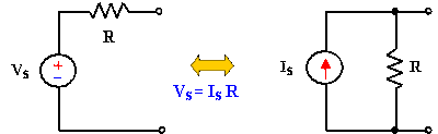
Source transformation is simplifying a circuit solution, especially with mixed sources, by transforming a voltage into a current source, and vice-versa. Finding a solution to a circuit can be difficult without using methods such as this to make the circuit appear simpler. Source transformation is another tool for simplifying circuits. Basic to these tools is the concept of equivalence.

A Source Transformation is the process of replacing a voltage source Vs in series with a resistor R by a current source Is in parallel with a resistor R, or vice-versa.

Source transformation requires that,

Vs = IsR or Is = Vs/R

Source transformation also applies to dependent sources, provided we carefully handle the dependent variable. As shown in below, a dependent voltage source in series with a resistor can be transformed to a dependent current source in parallel with the resistor or vice versa.

OVERVIEW AND INSIGHTS

Linearity Property talks about the voltage (v) and current (i), whereas voltage is directly proportional to the current, that is, when the voltage is increasing the current also increasing and vice-versa. I also learned that Source Transformation is only applicable to simple circuits and not in a complicated circuits.

Source Transformation can be applied if and only if the voltage is in series with the resistor and/or the current is in parallel with the resistor.

In Source Transformation you need to check the polarity of the source, when the polarity of the voltage source has a positive on top therefore the resulting current source is pointing upward and vice-versa. Also when the voltage source is dependent therefore the resulting current is also dependent, same calculations with independent sources.

Linggo, Agosto 10, 2014

Mesh Analysis

Mesh Analysis

Mesh analysis (or the mesh current method) is a method that is used to solve planar circuits for the currents (and indirectly the voltages) at any place in the circuit. Planar circuits are circuits that can be drawn on a plane surface with no wires crossing each other. A more general technique, called loop analysis (with the corresponding network variables called loop currents) can be applied to any circuit, planar or not. Mesh analysis and loop analysis both make use of Kirchhoff’s voltage law to arrive at a set of equations guaranteed to be solvable if the circuit has a solution. Mesh analysis is usually easier to use when the circuit is planar, compared to loop analysis.

Steps to determine mesh currents:

1.) Assign mesh currents i1,i2, . . . . in to the n meshes.

2.) Apply KVL to each of the n meshes. Use Ohm’s law to express the voltages in terms of the mesh currents.

3.) Solve the resulting n simultaneous equations to get the mesh currents

Essential meshes of the planar circuit labeled 1, 2, and 3. R₁, R₂, R₃, 1/sc, and Ls represent the impedance of the resistors, capacitor, and inductor values in the s-domain. V_s and i_s are the values of the voltage source and current source, respectively.

Circuit with mesh currents labeled as i₁, i₂, and i₃. The arrows show the direction of the mesh current.

What is Super mesh?

A super mesh occurs when a current source is contained between two essential meshes. The circuit is first treated as if the current source is not there. This leads to one equation that incorporates two mesh currents. Once this equation is formed, an equation is needed that relates the two mesh currents with the current source. This will be an equation where the current source is equal to one of the mesh currents minus the other. The following is a simple example of dealing with a super mesh.

$\begin{cases} \text{Mesh 1, 2: } -V_s + R_1I_1 + R_2I_2 = 0\\ \text{Current source: } I_s = I_2 - I_1 \end{cases} \,$

Circuit with a super mesh. Super mesh occurs because the current source is in between the essential meshes.

OVERVIEW AND INSIGHTS

A mesh current is a current that loops around and the equations are set solved in terms of them. A mesh current may not correspond to any physically flowing current, but the physical currents are easily found from them. It is usual practice to have all the mesh currents loop in the same direction. This helps prevent errors when writing out the equations. The convention is to have all the mesh currents looping in a clockwise direction.

in Mesh analysis it is a method that is used to solve planar circuits for the currents at any place in the circuit. Planar circuits are circuits that can be drawn on a plane.

From my own understanding a mesh I a loop that does not contain any other loop within it.

Electrical Circuits

Mga Pahina

Sabado, Oktubre 11, 2014

First Order Circuits

RL Circuits

RC Circuits

First Order Solution

Series RL

Series RC

Time Constant

Maximum Power Transfer Theorem, Capacitors and Inductors

Thevenin's and Norton's Theorem

Thevenin's Theorem

Norton's Theorem

Lunes, Agosto 25, 2014

Superposition Theorem

Linggo, Agosto 17, 2014

Linearity Property and Source Transformation

Linggo, Agosto 10, 2014

Mesh Analysis